文章目录
-
Python常用模块
-
time模块
-
时间戳
* 格式化时间
* 结构化时间
* 不同格式时间的转换
* 其他用法
- datetime模块
- random模块
- os模块
- sys模块
- json和pickle模块
-
序列化
* json
* pickle
-
hash是什么
* 撞库破解hash算法加密
-
日志级别
* 日志打印
* 应用
-
创建矩阵
* 获取矩阵的行列数
* 切割矩阵
* 矩阵元素替换
* 矩阵的合并
* 通过函数创建矩阵
-
arange
* linspace/logspace
* zeros/ones/eye/empty
* fromstring/fromfunction
-
普通矩阵运算
* 常用矩阵运算函数
1
2
3
4
5
| 1 * 矩阵的点乘
2 * 矩阵的转置
3 * 矩阵的逆
4 * 矩阵其他操作
5 |
-
最大最小值
* 平均值
* 方差
* 标准差
* 中位数
* 矩阵求和
* 累加和
1
2
| 1 * numpy.random生成随机数
2 |
-
Series
* DataFrame
* DataFrame属性
* DataFrame取值
-
loc/iloc
* 使用逻辑判断取值
1
2
3
4
5
6
7
| 1 * DataFrame值替换
2 * 读取CSV文件
3 * 处理丢失数据
4 * 导入导出数据
5 * 合并数据
6 * 读取sql语句
7 |
-
条形图
* 直方图
* 折线图
* 散点图+直线图
Python常用模块
time模块
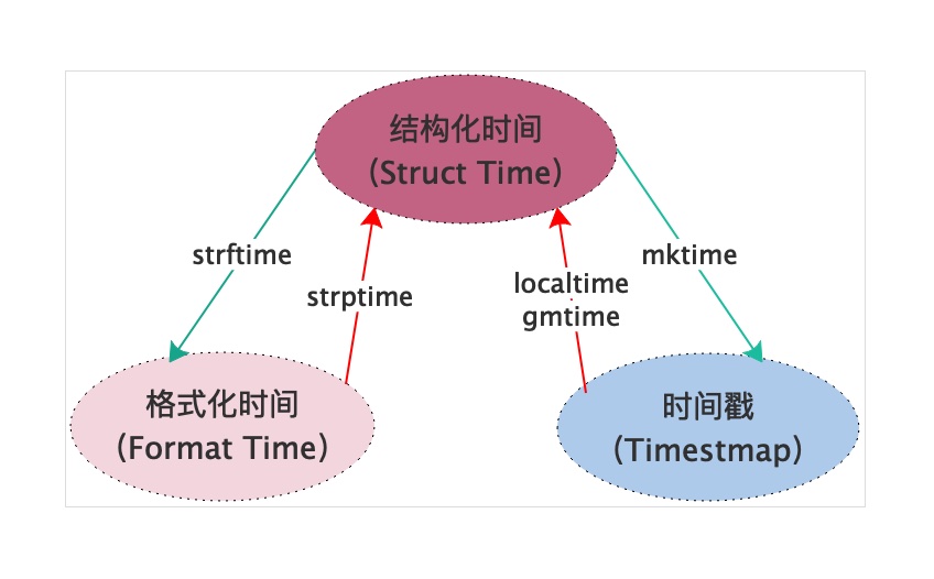
时间戳
时间戳(timestamp):时间戳表示的是从1970年1月1日00:00:00开始按秒计算的偏移量。
1
2
3
4
| 1time_stamp = time.time()
2print(time_stamp, type(time_stamp))
3
4 |
1
2
3
| 11552551519.291029 <class 'float'>
2
3 |
格式化时间
格式化的时间字符串(format string):格式化时间表示的是普通的字符串格式的时间。
1
2
3
4
| 1format_time = time.strftime("%Y-%m-%d %X")
2print(format_time, type(format_time))
3
4 |
1
2
3
| 12019-03-07 16:22:11 <class 'str'>
2
3 |
结构化时间
结构化的时间(struct time):struct_time元组共有9个元素共九个元素,分别为(年,月,日,时,分,秒,一年中第几周,一年中第几天,夏令时)
1
2
3
4
| 1print('本地时区的struct_time:\n{}'.format(time.localtime()))
2print('UTC时区的struct_time:\n{}'.format(time.gmtime()))
3
4 |
1
2
3
4
5
6
| 1本地时区的struct_time:
2time.struct_time(tm_year=2019, tm_mon=3, tm_mday=7, tm_hour=16, tm_min=22, tm_sec=11, tm_wday=3, tm_yday=66, tm_isdst=0)
3UTC时区的struct_time:
4time.struct_time(tm_year=2019, tm_mon=3, tm_mday=7, tm_hour=8, tm_min=22, tm_sec=11, tm_wday=3, tm_yday=66, tm_isdst=0)
5
6 |
1
2
3
4
| 1# 结构化时间的基准时间
2print(time.localtime(0))
3
4 |
1
2
3
| 1time.struct_time(tm_year=1970, tm_mon=1, tm_mday=1, tm_hour=8, tm_min=0, tm_sec=0, tm_wday=3, tm_yday=1, tm_isdst=0)
2
3 |
1
2
3
4
| 1# 结构化时间的基准时间上增加一年时间
2print(time.localtime(3600*24*365))
3
4 |
1
2
3
| 1time.struct_time(tm_year=1971, tm_mon=1, tm_mday=1, tm_hour=8, tm_min=0, tm_sec=0, tm_wday=4, tm_yday=1, tm_isdst=0)
2
3 |
不同格式时间的转换

如上图所示,我们总能通过某些方法在结构化时间-格式化时间-时间戳三者之间进行转换,下面我们将用代码展示如何通过这些方法转换时间格式。
1
2
3
4
5
| 1# 结构化时间
2now_time = time.localtime()
3print(now_time)
4
5 |
1
2
3
| 1time.struct_time(tm_year=2019, tm_mon=3, tm_mday=7, tm_hour=16, tm_min=22, tm_sec=11, tm_wday=3, tm_yday=66, tm_isdst=0)
2
3 |
1
2
3
4
| 1# 把结构化时间转换为时间戳格式
2print(time.mktime(now_time))
3
4 |
1
2
3
4
5
| 1# 把结构化时间转换为格式化时间
2# %Y年-%m月-%d天 %X时分秒=%H时:%M分:%S秒
3print(time.strftime("%Y-%m-%d %X", now_time))
4
5 |
1
2
3
| 12019-03-07 16:22:11
2
3 |
1
2
3
4
| 1# 把格式化时间化为结构化时间,它和strftime()是逆操作
2print(time.strptime('2013-05-20 13:14:52', '%Y-%m-%d %X'))
3
4 |
1
2
3
| 1time.struct_time(tm_year=2013, tm_mon=5, tm_mday=20, tm_hour=13, tm_min=14, tm_sec=52, tm_wday=0, tm_yday=140, tm_isdst=-1)
2
3 |
1
2
3
4
| 1# 把结构化时间表示为这种形式:'Sun Jun 20 23:21:05 1993'。
2print(time.asctime())
3
4 |
1
2
3
| 1Thu Mar 7 16:22:11 2019
2
3 |
1
2
3
4
| 1# 如果没有参数,将会将time.localtime()作为参数传入。
2print(time.asctime(time.localtime()))
3
4 |
1
2
3
| 1Thu Mar 7 16:22:11 2019
2
3 |
1
2
3
4
| 1# 把一个时间戳转化为time.asctime()的形式。
2print(time.ctime())
3
4 |
1
2
3
| 1Thu Mar 7 16:22:11 2019
2
3 |
1
2
3
4
| 1# 如果参数未给或者为None的时候,将会默认time.time()为参数。它的作用相当于time.asctime(time.localtime(secs))。
2print(time.ctime(time.time()))
3
4 |
1
2
3
| 1Thu Mar 7 16:22:11 2019
2
3 |
其他用法
1
2
3
4
5
6
7
8
| 1# 推迟指定的时间运行,单位为秒
2start = time.time()
3time.sleep(3)
4end = time.time()
5
6print(end-start)
7
8 |
1
2
3
| 13.0005428791046143
2
3 |
datetime模块
1
2
3
4
| 1# datetime模块可以看成是时间加减的模块
2import datetime
3
4 |
1
2
3
4
| 1# 返回当前时间
2print(datetime.datetime.now())
3
4 |
1
2
3
| 12019-03-07 16:22:14.544130
2
3 |
1
2
3
| 1print(datetime.date.fromtimestamp(time.time()))
2
3 |
1
2
3
4
| 1# 当前时间+3天
2print(datetime.datetime.now() + datetime.timedelta(3))
3
4 |
1
2
3
| 12019-03-10 16:22:14.560599
2
3 |
1
2
3
4
| 1# 当前时间-3天
2print(datetime.datetime.now() + datetime.timedelta(-3))
3
4 |
1
2
3
| 12019-03-04 16:22:14.568473
2
3 |
1
2
3
4
| 1# 当前时间-3小时
2print(datetime.datetime.now() + datetime.timedelta(hours=3))
3
4 |
1
2
3
| 12019-03-07 19:22:14.575881
2
3 |
1
2
3
4
| 1# 当前时间+30分钟
2print(datetime.datetime.now() + datetime.timedelta(minutes=30))
3
4 |
1
2
3
| 12019-03-07 16:52:14.585432
2
3 |
1
2
3
4
5
| 1# 时间替换
2c_time = datetime.datetime.now()
3print(c_time.replace(minute=20, hour=5, second=13))
4
5 |
1
2
3
| 12019-03-07 05:20:13.595493
2
3 |
random模块
1
2
3
4
| 1# 大于0且小于1之间的小数
2print(random.random())
3
4 |
1
2
3
| 10.25435092120631386
2
3 |
1
2
3
4
| 1# 大于等于1且小于等于3之间的整数
2print(random.randint(1, 3))
3
4 |
1
2
3
4
| 1# 大于等于1且小于3之间的整数
2print(random.randrange(1, 3))
3
4 |
1
2
3
4
| 1# 大于1小于3的小数,如1.927109612082716
2print(random.uniform(1, 3))
3
4 |
1
2
3
| 12.718804989532962
2
3 |
1
2
3
4
| 1# 列表内的任意一个元素,即1或者‘23’或者[4,5]
2print(random.choice([1, '23', [4, 5]]))
3
4 |
1
2
3
4
| 1# random.sample([], n),列表元素任意n个元素的组合,示例n=2
2print(random.sample([1, '23', [4, 5]], 2))
3
4 |
1
2
3
| 1[[4, 5], '23']
2
3 |
1
2
3
4
5
6
| 1lis = [1, 3, 5, 7, 9]
2# 打乱l的顺序,相当于"洗牌"
3random.shuffle(lis)
4print(lis)
5
6 |
os模块
os模块负责程序与操作系统交互。
os.getcwd()
获取当前工作目录,即当前python脚本工作的目录路径
os.chdir(“dirname”)
改变当前脚本工作目录;相当于shell下cd
os.curdir
返回当前目录: (’.’)
os.pardir
获取当前目录的父目录字符串名:(’…’)
os.makedirs(‘dirname1/dirname2’)
可生成多层递归目录
os.removedirs(‘dirname1’)
若目录为空,则删除,并递归到上一级目录,如若也为空,则删除,依此类推
os.mkdir(‘dirname’)
生成单级目录;相当于shell中mkdir dirname
os.rmdir(‘dirname’)
删除单级空目录,若目录不为空则无法删除,报错;相当于shell中rmdir dirname
os.listdir(‘dirname’)
列出指定目录下的所有文件和子目录,包括隐藏文件,并以列表方式打印
os.remove()
删除一个文件
os.rename(“oldname”,“newname”)
重命名文件/目录
os.stat(‘path/filename’)
获取文件/目录信息
os.sep
输出操作系统特定的路径分隔符,win下为"",Linux下为"/"
os.linesep
输出当前平台使用的行终止符,win下为"\t\n",Linux下为"\n"
os.pathsep
输出用于分割文件路径的字符串 win下为;,Linux下为:
os.name
输出字符串指示当前使用平台。win->‘nt’; Linux->‘posix’
os.system(“bash command”)
运行shell命令,直接显示
os.environ
获取系统环境变量
os.path.abspath(path)
返回path规范化的绝对路径
os.path.split(path)
将path分割成目录和文件名二元组返回
os.path.dirname(path)
返回path的目录。其实就是os.path.split(path)的第一个元素
os.path.basename(path)
返回path最后的文件名。如何path以/或\结尾,那么就会返回空值。即os.path.split(path)的第二个元素
os.path.exists(path)
如果path存在,返回True;如果path不存在,返回False
os.path.isabs(path)
如果path是绝对路径,返回True
os.path.isfile(path)
如果path是一个存在的文件,返回True。否则返回False
os.path.isdir(path)
如果path是一个存在的目录,则返回True。否则返回False
os.path.join(path1[, path2[, …]])
将多个路径组合后返回,第一个绝对路径之前的参数将被忽略
os.path.getatime(path)
返回path所指向的文件或者目录的最后存取时间
os.path.getmtime(path)
返回path所指向的文件或者目录的最后修改时间
os.path.getsize(path) 返回path的大小
sys模块
sys模块负责程序与Python解释器进行交互。
sys.argv
命令行参数List,第一个元素是程序本身路径
sys.modules.keys()
返回所有已经导入的模块列表
sys.exc_info()
获取当前正在处理的异常类,exc_type、exc_value、exc_traceback当前处理的异常详细信息
sys.exit(n)
退出程序,正常退出时exit(0)
sys.hexversion
获取Python解释程序的版本值,16进制格式如:0x020403F0
sys.version
获取Python解释程序的版本信息
sys.maxint
最大的Int值
sys.maxunicode
最大的Unicode值
sys.modules
返回系统导入的模块字段,key是模块名,value是模块
sys.path
返回模块的搜索路径,初始化时使用PYTHONPATH环境变量的值
sys.platform
返回操作系统平台名称
sys.stdout
标准输出
sys.stdin
标准输入
sys.stderr
错误输出
sys.exc_clear()
用来清除当前线程所出现的当前的或最近的错误信息
sys.exec_prefix
返回平台独立的python文件安装的位置
sys.byteorder
本地字节规则的指示器,big-endian平台的值是’big’,little-endian平台的值是’little’
sys.copyright
记录python版权相关的东西
sys.api_version
解释器的C的API版本
json和pickle模块
序列化
把对象(变量)从内存中变成可存储或传输的过程称之为序列化,在Python中叫pickling,在其他语言中也被称之为serialization,marshalling,flattening。
序列化的优点:
- 持久保存状态:内存是无法永久保存数据的,当程序运行了一段时间,我们断电或者重启程序,内存中关于这个程序的之前一段时间的数据(有结构)都被清空了。但是在断电或重启程序之前将程序当前内存中所有的数据都保存下来(保存到文件中),以便于下次程序执行能够从文件中载入之前的数据,然后继续执行,这就是序列化。
- 跨平台数据交互:序列化时不仅可以把序列化后的内容写入磁盘,还可以通过网络传输到别的机器上,如果收发的双方约定好实用一种序列化的格式,那么便打破了平台/语言差异化带来的限制,实现了跨平台数据交互。
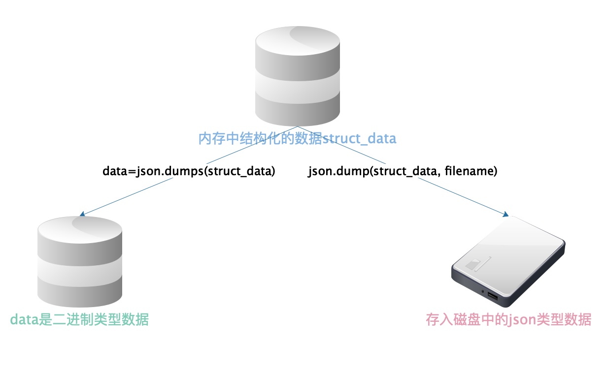
json
Json序列化并不是python独有的,json序列化在java等语言中也会涉及到,因此使用json序列化能够达到跨平台传输数据的目的。
json数据类型和python数据类型对应关系表
{}
dict
[]
list
“string”
str
520.13
int或float
true/false
True/False
null
None
json模块序列化和反序列化的一个过程如下图所示
1
2
3
4
| 1struct_data = {'name': 'json', 'age': 23, 'sex': 'male'}
2print(struct_data, type(struct_data))
3
4 |
1
2
3
| 1{'name': 'json', 'age': 23, 'sex': 'male'} <class 'dict'>
2
3 |
1
2
3
4
| 1data = json.dumps(struct_data)
2print(data, type(data))
3
4 |
1
2
3
| 1{"name": "json", "age": 23, "sex": "male"} <class 'str'>
2
3 |
1
2
3
4
5
| 1# 注意:无论数据是怎样创建的,只要满足json格式(如果是字典,则字典内元素都是双引号),就可以json.loads出来,不一定非要dumps的数据才能loads
2data = json.loads(data)
3print(data, type(data))
4
5 |
1
2
3
| 1{'name': 'json', 'age': 23, 'sex': 'male'} <class 'dict'>
2
3 |
1
2
3
4
5
| 1# 序列化
2with open('Json序列化对象.json', 'w') as fw:
3 json.dump(struct_data, fw)
4
5 |
1
2
3
4
5
6
| 1# 反序列化
2with open('Json序列化对象.json') as fr:
3 data = json.load(fr)
4print(data)
5
6 |
1
2
3
| 1{'name': 'json', 'age': 23, 'sex': 'male'}
2
3 |
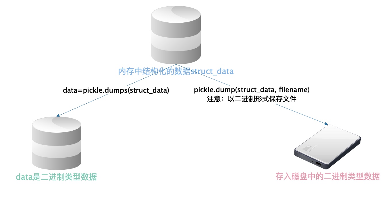
pickle
Pickle序列化和所有其他编程语言特有的序列化问题一样,它只能用于Python,并且可能不同版本的Python彼此都不兼容,因此,只能用Pickle保存那些不重要的数据,即不能成功地反序列化也没关系。但是pickle的好处是可以存储Python中的所有的数据类型,包括对象,而json不可以。
pickle模块序列化和反序列化的过程如下图所示
1
2
3
4
| 1struct_data = {'name': 'json', 'age': 23, 'sex': 'male'}
2print(struct_data, type(struct_data))
3
4 |
1
2
3
| 1{'name': 'json', 'age': 23, 'sex': 'male'} <class 'dict'>
2
3 |
1
2
3
4
| 1data = pickle.dumps(struct_data)
2print(data, type(data))
3
4 |
1
2
3
| 1b'\x80\x03}q\x00(X\x04\x00\x00\x00nameq\x01X\x04\x00\x00\x00jsonq\x02X\x03\x00\x00\x00ageq\x03K\x17X\x03\x00\x00\x00sexq\x04X\x04\x00\x00\x00maleq\x05u.' <class 'bytes'>
2
3 |
1
2
3
4
| 1data = pickle.loads(data)
2print(data, type(data))
3
4 |
1
2
3
| 1{'name': 'json', 'age': 23, 'sex': 'male'} <class 'dict'>
2
3 |
1
2
3
4
5
| 1# 序列化(注意:pickle模块需要使用二进制存储,即'wb'模式存储)
2with open('Pickle序列化对象.pkl', 'wb') as fw:
3 pickle.dump(struct_data, fw)
4
5 |
1
2
3
4
5
6
| 1# 反序列化
2with open('Pickle序列化对象.pkl', 'rb') as fr:
3 pickle = pickle.load(fr)
4print(data)
5
6 |
1
2
3
| 1{'name': 'json', 'age': 23, 'sex': 'male'}
2
3 |
hashlib模块
hash是什么
hash是一种算法(Python3.版本里使用hashlib模块代替了md5模块和sha模块,主要提供 SHA1、SHA224、SHA256、SHA384、SHA512、MD5 算法),该算法接受传入的内容,经过运算得到一串hash值。
hash值的特点:
- 只要传入的内容一样,得到的hash值一样,可用于非明文密码传输时密码校验
- 不能由hash值返解成内容,即可以保证非明文密码的安全性
- 只要使用的hash算法不变,无论校验的内容有多大,得到的hash值长度是固定的,可以用于对文本的哈希处理
hash算法其实可以看成如下图所示的一座工厂,工厂接收你送来的原材料,经过加工返回的产品就是hash值
1
2
3
4
5
6
| 1m = hashlib.md5()
2
3m.update('hello'.encode('utf8'))
4print(m.hexdigest())
5
6 |
1
2
3
| 15d41402abc4b2a76b9719d911017c592
2
3 |
1
2
3
4
| 1m.update('hash'.encode('utf8'))
2print(m.hexdigest())
3
4 |
1
2
3
| 197fa850988687b8ceb12d773347f7712
2
3 |
1
2
3
4
5
| 1m2 = hashlib.md5()
2m2.update('hellohash'.encode('utf8'))
3print(m2.hexdigest())
4
5 |
1
2
3
| 197fa850988687b8ceb12d773347f7712
2
3 |
1
2
3
4
5
| 1m3 = hashlib.md5()
2m3.update('hello'.encode('utf8'))
3print(m3.hexdigest())
4
5 |
1
2
3
| 15d41402abc4b2a76b9719d911017c592
2
3 |
撞库破解hash算法加密
hash加密算法虽然看起来很厉害,但是他是存在一定缺陷的,即可以通过撞库可以反解,如下代码所示。
1
2
3
4
5
6
7
8
9
10
11
12
13
14
15
16
17
18
19
20
21
22
23
24
25
26
27
28
29
30
31
32
| 1import hashlib
2
3# 假定我们知道hash的微信会设置如下几个密码
4pwd_list = [
5 'hash3714',
6 'hash1313',
7 'hash94139413',
8 'hash123456',
9 '123456hash',
10 'h123ash',
11]
12
13
14def make_pwd_dic(pwd_list):
15 dic = {}
16 for pwd in pwd_list:
17 m = hashlib.md5()
18 m.update(pwd.encode('utf-8'))
19 dic[pwd] = m.hexdigest()
20 return dic
21
22
23def break_code(hash_pwd, pwd_dic):
24 for k, v in pwd_dic.items():
25 if v == hash_pwd:
26 print('hash的微信的密码是===>\033[46m%s\033[0m' % k)
27
28
29hash_pwd = '0562b36c3c5a3925dbe3c4d32a4f2ba2'
30break_code(hash_pwd, make_pwd_dic(pwd_list))
31
32 |
1
2
3
| 1hash的微信的密码是===>[46mhash123456[0m
2
3 |
为了防止密码被撞库,我们可以使用python中的另一个hmac 模块,它内部对我们创建key和内容做过某种处理后再加密。
如果要保证hmac模块最终结果一致,必须保证:
-
hmac.new括号内指定的初始key一样
-
无论update多少次,校验的内容累加到一起是一样的内容
1
2
3
4
5
6
7
8
9
| 1import hmac
2
3# 注意hmac模块只接受二进制数据的加密
4h1 = hmac.new(b'hash')
5h1.update(b'hello')
6h1.update(b'world')
7print(h1.hexdigest())
8
9 |
1
2
3
| 1905f549c5722b5850d602862c34a763e
2
3 |
1
2
3
4
5
| 1h2 = hmac.new(b'hash')
2h2.update(b'helloworld')
3print(h2.hexdigest())
4
5 |
1
2
3
| 1905f549c5722b5850d602862c34a763e
2
3 |
1
2
3
4
| 1h3 = hmac.new(b'hashhelloworld')
2print(h3.hexdigest())
3
4 |
1
2
3
| 1a7e524ade8ac5f7f33f3a39a8f63fd25
2
3 |
logging模块
日志级别
- CRITICAL = 50
- ERROR = 40
- WARNING = 30
- INFO = 20
- DEBUG = 10
- NOTSET = 0
日志打印
1
2
3
4
5
6
7
8
9
10
| 1import logging
2
3# 默认级别为warning,错误级别达到warning以上的才会被打印
4# logging.debug('调试debug')
5# logging.info('消息info')
6# logging.warning('警告warn')
7# logging.error('错误error')
8# logging.critical('严重critical')
9
10 |
1
2
3
4
5
6
7
| 1[DEBUG][2019-03-07 16:22:14,853][<ipython-input-260-f62127333de0>:4]调试debug
2[INFO][2019-03-07 16:22:14,857][<ipython-input-260-f62127333de0>:5]消息info
3[WARNING][2019-03-07 16:22:14,858][<ipython-input-260-f62127333de0>:6]警告warn
4[ERROR][2019-03-07 16:22:14,860][<ipython-input-260-f62127333de0>:7]错误error
5[CRITICAL][2019-03-07 16:22:14,862][<ipython-input-260-f62127333de0>:8]严重critical
6
7 |
应用
1
2
3
4
5
6
7
8
9
10
11
12
13
14
15
16
17
18
19
20
21
22
23
24
25
26
27
28
29
30
31
32
33
34
35
36
37
38
39
40
41
42
43
44
45
46
47
48
49
50
51
52
53
54
55
56
57
58
59
60
61
62
63
64
65
66
67
68
69
70
71
72
73
74
75
76
77
| 1# logging文件配置
2import os
3import logging.config
4
5# 定义三种日志输出格式 开始
6standard_format = '[%(asctime)s][%(threadName)s:%(thread)d][task_id:%(name)s][%(filename)s:%(lineno)d]' \
7 '[%(levelname)s][%(message)s]' # 其中name为getlogger指定的名字
8simple_format = '[%(levelname)s][%(asctime)s][%(filename)s:%(lineno)d]%(message)s'
9id_simple_format = '[%(levelname)s][%(asctime)s] %(message)s'
10
11
12logfile_dir = 'os.path.dirname(os.path.abspath(__file__))' # log文件的目录
13
14logfile_name = 'logfile.log' # log文件名
15
16# 如果不存在定义的日志目录就创建一个
17if not os.path.isdir(logfile_dir):
18 os.mkdir(logfile_dir)
19
20# log文件的全路径
21logfile_path = os.path.join(logfile_dir, logfile_name)
22
23# log配置字典
24LOGGING_DIC = {
25 'version': 1,
26 # 是否删除已经存在的日志
27 'disable_existing_loggers': False,
28 # 日志格式
29 'formatters': {
30 'standard': {
31 'format': standard_format
32 },
33 'simple': {
34 'format': simple_format
35 },
36 },
37 'filters': {},
38 'handlers': {
39 # 打印到终端的日志
40 'console': {
41 'level': 'DEBUG',
42 'class': 'logging.StreamHandler', # 打印到屏幕
43 'formatter': 'simple'
44 },
45 # 打印到文件的日志,收集info及以上的日志
46 'default': {
47 'level': 'DEBUG',
48 'class': 'logging.handlers.RotatingFileHandler', # 保存到文件
49 'formatter': 'standard',
50 'filename': logfile_path, # 日志文件
51 'maxBytes': 1024*1024*5, # 日志大小 5M
52 'backupCount': 5,
53 'encoding': 'utf-8', # 日志文件的编码
54 },
55 },
56 'loggers': {
57 # logging.getLogger(__name__)拿到的logger配置
58 '': {
59 # 这里把上面定义的两个handler都加上,即log数据既写入文件又打印到屏幕
60 'handlers': ['default', 'console'],
61 'level': 'DEBUG',
62 'propagate': True, # 向上(更高level的logger)传递
63 },
64 },
65}
66
67
68def load_my_logging_cfg():
69 logging.config.dictConfig(LOGGING_DIC) # 导入上面定义的logging配置
70 logger = logging.getLogger(__name__) # 生成一个log实例
71 logger.info('It works!') # 记录该文件的运行状态
72
73
74if __name__ == '__main__':
75 load_my_logging_cfg()
76
77 |
1
2
3
4
5
6
7
8
9
10
11
12
13
14
15
16
17
18
19
20
21
22
23
24
25
| 1# 测试使用日志文件配置
2
3import time
4import logging
5import my_logging # 导入自定义的logging配置,上面的日志配置文件
6
7logger = logging.getLogger(__name__) # 生成logger实例
8
9
10def demo():
11 logger.debug("start range. time:{}".format(time.time()))
12 logger.info("中文测试开始。")
13 for i in range(10):
14 logger.debug("i:{}".format(i))
15 time.sleep(0.2)
16 else:
17 logger.debug("over range. time:{}".format(time.time()))
18 logger.info("中文测试结束。")
19
20
21if __name__ == "__main__":
22 my_logging.load_my_logging_cfg() # 在你程序文件的入口加载自定义logging配置
23 demo()
24
25 |
numpy模块
numpy官方文档:https://docs.scipy.org/doc/numpy/reference/?v=20190307135750
numpy是Python的一种开源的数值计算扩展库。这种库可用来存储和处理大型矩阵,比Python自身的嵌套列表结构要高效的多(该结构也可以用来表示矩阵)。
numpy库有两个作用:
- 区别于list列表,提供了数组操作、数组运算、以及统计分布和简单的数学模型
- 计算速度快,甚至要由于python内置的简单运算,使得其成为pandas、sklearn等模块的依赖包。高级的框架如TensorFlow、PyTorch等,其数组操作也和numpy非常相似。
创建矩阵
矩阵即numpy的ndarray对象,创建矩阵就是把一个列表传入np.array()方法。
1
2
3
| 1import numpy as np
2
3 |
1
2
3
4
5
| 1# 创建一维的ndarray对象
2arr = np.array([1, 2, 3])
3print(arr, type(arr))
4
5 |
1
2
3
| 1[1 2 3] <class 'numpy.ndarray'>
2
3 |
1
2
3
4
| 1# 创建二维的ndarray对象
2print(np.array([[1, 2, 3], [4, 5, 6]]))
3
4 |
1
2
3
4
| 1[[1 2 3]
2 [4 5 6]]
3
4 |
1
2
3
4
| 1# 创建三维的ndarray对象
2print(np.array([[1, 2, 3], [4, 5, 6], [7, 8, 9]]))
3
4 |
1
2
3
4
5
| 1[[1 2 3]
2 [4 5 6]
3 [7 8 9]]
4
5 |
获取矩阵的行列数
1
2
3
4
| 1arr = np.array([[1, 2, 3], [4, 5, 6]])
2print(arr)
3
4 |
1
2
3
4
| 1[[1 2 3]
2 [4 5 6]]
3
4 |
1
2
3
4
| 1# 获取矩阵的行和列构成的数组
2print(arr.shape)
3
4 |
1
2
3
4
| 1# 获取矩阵的行
2print(arr.shape[0])
3
4 |
1
2
3
4
| 1# 获取矩阵的列
2print(arr.shape[1])
3
4 |
切割矩阵
切分矩阵类似于列表的切割,但是与列表的切割不同的是,矩阵的切割涉及到行和列的切割,但是两者切割的方式都是从索引0开始,并且取头不取尾。
1
2
3
4
| 1arr = np.array([[1, 2, 3, 4], [5, 6, 7, 8], [9, 10, 11, 12]])
2print(arr)
3
4 |
1
2
3
4
5
| 1[[ 1 2 3 4]
2 [ 5 6 7 8]
3 [ 9 10 11 12]]
4
5 |
1
2
3
4
| 1# 取所有元素
2print(arr[:, :])
3
4 |
1
2
3
4
5
| 1[[ 1 2 3 4]
2 [ 5 6 7 8]
3 [ 9 10 11 12]]
4
5 |
1
2
3
4
| 1# 取第一行的所有元素
2print(arr[:1, :])
3
4 |
1
2
3
4
| 1# 取第一行的所有元素
2print(arr[0, [0, 1, 2, 3]])
3
4 |
1
2
3
4
| 1# 取第一列的所有元素
2print(arr[:, :1])
3
4 |
1
2
3
4
5
| 1[[1]
2 [5]
3 [9]]
4
5 |
1
2
3
4
| 1# 取第一列的所有元素
2print(arr[(0, 1, 2), 0])
3
4 |
1
2
3
4
| 1# 取第一行第一列的元素
2print(arr[(0, 1, 2), 0])
3
4 |
1
2
3
4
| 1# 取第一行第一列的元素
2print(arr[0, 0])
3
4 |
1
2
3
4
| 1# 取大于5的元素,返回一个数组
2print(arr[arr > 5])
3
4 |
1
2
3
| 1[ 6 7 8 9 10 11 12]
2
3 |
1
2
3
4
| 1# 矩阵按运算符取元素的原理,即通过arr > 5生成一个布尔矩阵
2print(arr > 5)
3
4 |
1
2
3
4
5
| 1[[False False False False]
2 [False True True True]
3 [ True True True True]]
4
5 |
矩阵元素替换
矩阵元素的替换,类似于列表元素的替换,并且矩阵也是一个可变类型的数据,即如果对矩阵进行替换操作,会修改原矩阵的元素,所以下面我们用.copy()方法举例矩阵元素的替换。
1
2
3
4
| 1arr = np.array([[1, 2, 3, 4], [5, 6, 7, 8], [9, 10, 11, 12]])
2print(arr)
3
4 |
1
2
3
4
5
| 1[[ 1 2 3 4]
2 [ 5 6 7 8]
3 [ 9 10 11 12]]
4
5 |
1
2
3
4
5
6
| 1# 取第一行的所有元素,并且让第一行的元素都为0
2arr1 = arr.copy()
3arr1[:1, :] = 0
4print(arr1)
5
6 |
1
2
3
4
5
| 1[[ 0 0 0 0]
2 [ 5 6 7 8]
3 [ 9 10 11 12]]
4
5 |
1
2
3
4
5
6
| 1# 取所有大于5的元素,并且让大于5的元素为0
2arr2 = arr.copy()
3arr2[arr > 5] = 0
4print(arr2)
5
6 |
1
2
3
4
5
| 1[[1 2 3 4]
2 [5 0 0 0]
3 [0 0 0 0]]
4
5 |
1
2
3
4
5
6
| 1# 对矩阵清零
2arr3 = arr.copy()
3arr3[:, :] = 0
4print(arr3)
5
6 |
1
2
3
4
5
| 1[[0 0 0 0]
2 [0 0 0 0]
3 [0 0 0 0]]
4
5 |
矩阵的合并
1
2
3
4
| 1arr1 = np.array([[1, 2], [3, 4], [5, 6]])
2print(arr1)
3
4 |
1
2
3
4
5
| 1[[1 2]
2 [3 4]
3 [5 6]]
4
5 |
1
2
3
4
| 1arr2 = np.array([[7, 8], [9, 10], [11, 12]])
2print(arr2)
3
4 |
1
2
3
4
5
| 1[[ 7 8]
2 [ 9 10]
3 [11 12]]
4
5 |
1
2
3
4
| 1# 合并两个矩阵的行,注意使用hstack()方法合并矩阵,矩阵应该有相同的行,其中hstack的h表示horizontal水平的
2print(np.hstack((arr1, arr2)))
3
4 |
1
2
3
4
5
| 1[[ 1 2 7 8]
2 [ 3 4 9 10]
3 [ 5 6 11 12]]
4
5 |
1
2
3
4
| 1# 合并两个矩阵,其中axis=1表示合并两个矩阵的行
2print(np.concatenate((arr1, arr2), axis=1))
3
4 |
1
2
3
4
5
| 1[[ 1 2 7 8]
2 [ 3 4 9 10]
3 [ 5 6 11 12]]
4
5 |
1
2
3
4
| 1# 合并两个矩阵的列,注意使用vstack()方法合并矩阵,矩阵应该有相同的列,其中vstack的v表示vertical垂直的
2print(np.vstack((arr1, arr2)))
3
4 |
1
2
3
4
5
6
7
8
| 1[[ 1 2]
2 [ 3 4]
3 [ 5 6]
4 [ 7 8]
5 [ 9 10]
6 [11 12]]
7
8 |
1
2
3
4
| 1# 合并两个矩阵,其中axis=0表示合并两个矩阵的列
2print(np.concatenate((arr1, arr2), axis=0))
3
4 |
1
2
3
4
5
6
7
8
| 1[[ 1 2]
2 [ 3 4]
3 [ 5 6]
4 [ 7 8]
5 [ 9 10]
6 [11 12]]
7
8 |
通过函数创建矩阵
arange
1
2
3
4
| 1# 构造0-9的ndarray数组
2print(np.arange(10))
3
4 |
1
2
3
| 1[0 1 2 3 4 5 6 7 8 9]
2
3 |
1
2
3
4
| 1# 构造1-4的ndarray数组
2print(np.arange(1, 5))
3
4 |
1
2
3
4
| 1# 构造1-19且步长为2的ndarray数组
2print(np.arange(1, 20, 2))
3
4 |
1
2
3
| 1[ 1 3 5 7 9 11 13 15 17 19]
2
3 |
linspace/logspace
1
2
3
4
| 1# 构造一个等差数列,取头也取尾,从0取到20,取5个数
2print(np.linspace(0, 20, 5))
3
4 |
1
2
3
| 1[ 0. 5. 10. 15. 20.]
2
3 |
1
2
3
4
| 1# 构造一个等比数列,从10**0取到10**20,取5个数
2print(np.logspace(0, 20, 5))
3
4 |
1
2
3
4
| 1[ 1.00000000e+00 1.00000000e+05 1.00000000e+10 1.00000000e+15
2 1.00000000e+20]
3
4 |
zeros/ones/eye/empty
1
2
3
4
| 1# 构造3*4的全0矩阵
2print(np.zeros((3, 4)))
3
4 |
1
2
3
4
5
| 1[[ 0. 0. 0. 0.]
2 [ 0. 0. 0. 0.]
3 [ 0. 0. 0. 0.]]
4
5 |
1
2
3
4
| 1# 构造3*4的全1矩阵
2print(np.ones((3, 4)))
3
4 |
1
2
3
4
5
| 1[[ 1. 1. 1. 1.]
2 [ 1. 1. 1. 1.]
3 [ 1. 1. 1. 1.]]
4
5 |
1
2
3
4
| 1# 构造3个主元的单位矩阵
2print(np.eye(3))
3
4 |
1
2
3
4
5
| 1[[ 1. 0. 0.]
2 [ 0. 1. 0.]
3 [ 0. 0. 1.]]
4
5 |
1
2
3
4
| 1# 构造一个4*4的随机矩阵,里面的元素是随机生成的
2print(np.empty((4, 4)))
3
4 |
1
2
3
4
5
6
| 1[[ 1.72723371e-077 -2.68678116e+154 3.95252517e-323 0.00000000e+000]
2 [ 0.00000000e+000 0.00000000e+000 0.00000000e+000 0.00000000e+000]
3 [ 0.00000000e+000 0.00000000e+000 0.00000000e+000 0.00000000e+000]
4 [ 0.00000000e+000 0.00000000e+000 0.00000000e+000 1.17248833e-308]]
5
6 |
fromstring/fromfunction
1
2
3
4
5
6
| 1# fromstring通过对字符串的字符编码所对应ASCII编码的位置,生成一个ndarray对象
2s = 'abcdef'
3# np.int8表示一个字符的字节数为8
4print(np.fromstring(s, dtype=np.int8))
5
6 |
1
2
3
| 1[ 97 98 99 100 101 102]
2
3 |
1
2
3
4
5
6
7
8
9
| 1def func(i, j):
2 """其中i为矩阵的行,j为矩阵的列"""
3 return i*j
4
5
6# 使用函数对矩阵元素的行和列的索引做处理,得到当前元素的值,索引从0开始,并构造一个3*4的矩阵
7print(np.fromfunction(func, (3, 4)))
8
9 |
1
2
3
4
5
| 1[[ 0. 0. 0. 0.]
2 [ 0. 1. 2. 3.]
3 [ 0. 2. 4. 6.]]
4
5 |
矩阵的运算
普通矩阵运算
两个矩阵对应元素相加
两个矩阵对应元素相减
*
两个矩阵对应元素相乘
/
两个矩阵对应元素相除,如果都是整数则取商
%
两个矩阵对应元素相除后取余数
n
单个矩阵每个元素都取n次方,如2:每个元素都取平方
1
2
3
4
| 1arrarr1 = np.array([[1, 2], [3, 4], [5, 6]])
2print(arr1)
3
4 |
1
2
3
4
5
| 1[[1 2]
2 [3 4]
3 [5 6]]
4
5 |
1
2
3
4
| 1arr2 = np.array([[7, 8], [9, 10], [11, 12]])
2print(arr2)
3
4 |
1
2
3
4
5
| 1[[ 7 8]
2 [ 9 10]
3 [11 12]]
4
5 |
1
2
3
4
5
| 1[[ 8 10]
2 [12 14]
3 [16 18]]
4
5 |
1
2
3
4
5
| 1[[ 1 4]
2 [ 9 16]
3 [25 36]]
4
5 |
常用矩阵运算函数
np.sin(arr)
对矩阵arr中每个元素取正弦,$sin(x)$
np.cos(arr)
对矩阵arr中每个元素取余弦,$cos(x)$
np.tan(arr)
对矩阵arr中每个元素取正切,$tan(x)$
np.arcsin(arr)
对矩阵arr中每个元素取反正弦,$arcsin(x)$
np.arccos(arr)
对矩阵arr中每个元素取反余弦,$arccos(x)$
np.arctan(arr)
对矩阵arr中每个元素取反正切,$arctan(x)$
np.exp(arr)
对矩阵arr中每个元素取指数函数,$e^x$
np.sqrt(arr)
对矩阵arr中每个元素开根号$\sqrt{x}$
1
2
3
4
| 1arr = np.array([[1, 2, 3, 4], [5, 6, 7, 8], [9, 10, 11, 12]])
2print(arr)
3
4 |
1
2
3
4
5
| 1[[ 1 2 3 4]
2 [ 5 6 7 8]
3 [ 9 10 11 12]]
4
5 |
1
2
3
4
| 1# 对矩阵的所有元素取正弦
2print(np.sin(arr))
3
4 |
1
2
3
4
5
| 1[[ 0.84147098 0.90929743 0.14112001 -0.7568025 ]
2 [-0.95892427 -0.2794155 0.6569866 0.98935825]
3 [ 0.41211849 -0.54402111 -0.99999021 -0.53657292]]
4
5 |
1
2
3
4
| 1# 对矩阵的所有元素开根号
2print(np.sqrt(arr))
3
4 |
1
2
3
4
5
| 1[[ 1. 1.41421356 1.73205081 2. ]
2 [ 2.23606798 2.44948974 2.64575131 2.82842712]
3 [ 3. 3.16227766 3.31662479 3.46410162]]
4
5 |
1
2
3
4
| 1# 对矩阵的所有元素取反正弦,如果元素不在定义域内,则会取nan值
2print(np.arcsin(arr))
3
4 |
1
2
3
4
5
6
7
8
| 1[[ 1.57079633 nan nan nan]
2 [ nan nan nan nan]
3 [ nan nan nan nan]]
4
5
6/Applications/anaconda3/lib/python3.6/site-packages/ipykernel_launcher.py:2: RuntimeWarning: invalid value encountered in arcsin
7
8 |
矩阵的点乘
矩阵的点乘必须满足第一个矩阵的列数等于第二个矩阵的行数,即$m*n·{n*m}=m*m$。
1
2
3
4
| 1arr1 = np.array([[1, 2, 3], [4, 5, 6]])
2print(arr1.shape)
3
4 |
1
2
3
4
| 1arr2 = np.array([[7, 8], [9, 10], [11, 12]])
2print(arr2.shape)
3
4 |
1
2
3
4
5
| 1assert arr1.shape[0] == arr2.shape[1]
2# 2*3·3*2 = 2*2
3print(arr2.shape)
4
5 |
矩阵的转置
矩阵的转置,相当于矩阵的行和列互换。
1
2
3
4
| 1arr = np.array([[1, 2, 3], [4, 5, 6]])
2print(arr)
3
4 |
1
2
3
4
| 1[[1 2 3]
2 [4 5 6]]
3
4 |
1
2
3
| 1print(arr.transpose())
2
3 |
1
2
3
4
5
| 1[[1 4]
2 [2 5]
3 [3 6]]
4
5 |
1
2
3
4
5
| 1[[1 4]
2 [2 5]
3 [3 6]]
4
5 |
矩阵的逆
矩阵行和列相同时,矩阵才可逆。
1
2
3
4
| 1arr = np.array([[1, 2, 3], [4, 5, 6], [7, 8, 9]])
2print(arr)
3
4 |
1
2
3
4
5
| 1[[1 2 3]
2 [4 5 6]
3 [7 8 9]]
4
5 |
1
2
3
| 1print(np.linalg.inv(arr))
2
3 |
1
2
3
4
5
| 1[[ 3.15251974e+15 -6.30503948e+15 3.15251974e+15]
2 [ -6.30503948e+15 1.26100790e+16 -6.30503948e+15]
3 [ 3.15251974e+15 -6.30503948e+15 3.15251974e+15]]
4
5 |
1
2
3
4
5
| 1# 单位矩阵的逆是单位矩阵本身
2arr = np.eye(3)
3print(arr)
4
5 |
1
2
3
4
5
| 1[[ 1. 0. 0.]
2 [ 0. 1. 0.]
3 [ 0. 0. 1.]]
4
5 |
1
2
3
| 1print(np.linalg.inv(arr))
2
3 |
1
2
3
4
5
| 1[[ 1. 0. 0.]
2 [ 0. 1. 0.]
3 [ 0. 0. 1.]]
4
5 |
矩阵其他操作
最大最小值
1
2
3
4
| 1arr = np.array([[1, 2, 3], [4, 5, 6], [7, 8, 9]])
2print(arr)
3
4 |
1
2
3
4
5
| 1[[1 2 3]
2 [4 5 6]
3 [7 8 9]]
4
5 |
1
2
3
4
| 1# 获取矩阵所有元素中的最大值
2print(arr.max())
3
4 |
1
2
3
4
| 1# 获取矩阵所有元素中的最小值
2print(arr.min())
3
4 |
1
2
3
4
| 1# 获取举着每一行的最大值
2print(arr.max(axis=0))
3
4 |
1
2
3
4
| 1# 获取矩阵每一列的最大值
2print(arr.max(axis=1))
3
4 |
1
2
3
4
| 1# 获取矩阵最大元素的索引位置
2print(arr.argmax(axis=1))
3
4 |
平均值
1
2
3
4
| 1arr = np.array([[1, 2, 3], [4, 5, 6], [7, 8, 9]])
2print(arr)
3
4 |
1
2
3
4
5
| 1[[1 2 3]
2 [4 5 6]
3 [7 8 9]]
4
5 |
1
2
3
4
| 1# 获取矩阵所有元素的平均值
2print(arr.mean())
3
4 |
1
2
3
4
| 1# 获取矩阵每一列的平均值
2print(arr.mean(axis=0))
3
4 |
1
2
3
4
| 1# 获取矩阵每一行的平均值
2print(arr.mean(axis=1))
3
4 |
方差
方差公式为
$$mean(|x-x.mean()|^2)$$
其中x为矩阵。
1
2
3
4
| 1arr = np.array([[1, 2, 3], [4, 5, 6], [7, 8, 9]])
2print(arr)
3
4 |
1
2
3
4
5
| 1[[1 2 3]
2 [4 5 6]
3 [7 8 9]]
4
5 |
1
2
3
4
| 1# 获取矩阵所有元素的方差
2print(arr.var())
3
4 |
1
2
3
4
| 1# 获取矩阵每一列的元素的方差
2print(arr.var(axis=0))
3
4 |
1
2
3
4
| 1# 获取矩阵每一行的元素的方差
2print(arr.var(axis=1))
3
4 |
1
2
3
| 1[ 0.66666667 0.66666667 0.66666667]
2
3 |
标准差
标准差公式为
$$\sqrt{mean|x-x.mean()|^2} = \sqrt{x.var()}$$
1
2
3
4
| 1arr = np.array([[1, 2, 3], [4, 5, 6], [7, 8, 9]])
2print(arr)
3
4 |
1
2
3
4
5
| 1[[1 2 3]
2 [4 5 6]
3 [7 8 9]]
4
5 |
1
2
3
4
| 1# 获取矩阵所有元素的标准差
2print(arr.std())
3
4 |
1
2
3
4
| 1# 获取矩阵每一列的标准差
2print(arr.std(axis=0))
3
4 |
1
2
3
| 1[ 2.44948974 2.44948974 2.44948974]
2
3 |
1
2
3
4
| 1# 获取矩阵每一行的标准差
2print(arr.std(axis=1))
3
4 |
1
2
3
| 1[ 0.81649658 0.81649658 0.81649658]
2
3 |
中位数
1
2
3
4
| 1arr = np.array([[1, 2, 3], [4, 5, 6], [7, 8, 9]])
2print(arr)
3
4 |
1
2
3
4
5
| 1[[1 2 3]
2 [4 5 6]
3 [7 8 9]]
4
5 |
1
2
3
4
| 1# 获取矩阵所有元素的中位数
2print(np.median(arr))
3
4 |
1
2
3
4
| 1# 获取矩阵每一列的中位数
2print(np.median(arr, axis=0))
3
4 |
1
2
3
4
| 1# 获取矩阵每一行的中位数
2print(np.median(arr, axis=1))
3
4 |
矩阵求和
1
2
3
4
| 1arr = np.array([[1, 2, 3], [4, 5, 6], [7, 8, 9]])
2print(arr)
3
4 |
1
2
3
4
5
| 1[[1 2 3]
2 [4 5 6]
3 [7 8 9]]
4
5 |
1
2
3
4
| 1# 对矩阵的每一个元素求和
2print(arr.sum())
3
4 |
1
2
3
4
| 1# 对矩阵的每一列求和
2print(arr.sum(axis=0))
3
4 |
1
2
3
4
| 1# 对矩阵的每一行求和
2print(arr.sum(axis=1))
3
4 |
累加和
1
2
3
4
| 1arr = np.array([1, 2, 3, 4, 5])
2print(arr)
3
4 |
1
2
3
4
| 1# 第n个元素为前n-1个元素累加和
2print(arr.cumsum())
3
4 |
numpy.random生成随机数
rand($d_0, d_1, \cdots , d_n$)
产生均匀分布的随机数
$d_n$为第n维数据的维度
randn($d_0, d_1, \cdots , d_n$)
产生标准正态分布随机数
$d_n$为第n维数据的维度
randint(low[, high, size, dtype])
产生随机整数
low:最小值;high:最大值;size:数据个数
random_sample([size])
在$[0,1)$内产生随机数
size为随机数的shape,可以为元祖或者列表
choice(a[, size])
从arr中随机选择指定数据
arr为1维数组;size为数据形状
1
2
3
4
5
| 1# RandomState()方法会让数据值随机一次,之后都是相同的数据
2rs = np.random.RandomState(1)
3print(rs.rand(10))
4
5 |
1
2
3
4
5
| 1[ 4.17022005e-01 7.20324493e-01 1.14374817e-04 3.02332573e-01
2 1.46755891e-01 9.23385948e-02 1.86260211e-01 3.45560727e-01
3 3.96767474e-01 5.38816734e-01]
4
5 |
1
2
3
4
5
6
| 1# 构造3*4的均匀分布的矩阵
2# seed()方法会让数据值随机一次,之后都是相同的数据
3np.random.seed(1)
4print(np.random.rand(3, 4))
5
6 |
1
2
3
4
5
| 1[[ 4.17022005e-01 7.20324493e-01 1.14374817e-04 3.02332573e-01]
2 [ 1.46755891e-01 9.23385948e-02 1.86260211e-01 3.45560727e-01]
3 [ 3.96767474e-01 5.38816734e-01 4.19194514e-01 6.85219500e-01]]
4
5 |
1
2
3
4
| 1# 构造3*4*5的均匀分布的矩阵
2print(np.random.rand(3, 4, 5))
3
4 |
1
2
3
4
5
6
7
8
9
10
11
12
13
14
15
16
| 1[[[ 0.20445225 0.87811744 0.02738759 0.67046751 0.4173048 ]
2 [ 0.55868983 0.14038694 0.19810149 0.80074457 0.96826158]
3 [ 0.31342418 0.69232262 0.87638915 0.89460666 0.08504421]
4 [ 0.03905478 0.16983042 0.8781425 0.09834683 0.42110763]]
5
6 [[ 0.95788953 0.53316528 0.69187711 0.31551563 0.68650093]
7 [ 0.83462567 0.01828828 0.75014431 0.98886109 0.74816565]
8 [ 0.28044399 0.78927933 0.10322601 0.44789353 0.9085955 ]
9 [ 0.29361415 0.28777534 0.13002857 0.01936696 0.67883553]]
10
11 [[ 0.21162812 0.26554666 0.49157316 0.05336255 0.57411761]
12 [ 0.14672857 0.58930554 0.69975836 0.10233443 0.41405599]
13 [ 0.69440016 0.41417927 0.04995346 0.53589641 0.66379465]
14 [ 0.51488911 0.94459476 0.58655504 0.90340192 0.1374747 ]]]
15
16 |
1
2
3
4
| 1# 构造3*4的正态分布的矩阵
2print(np.random.randn(3, 4))
3
4 |
1
2
3
4
5
| 1[[ 0.30017032 -0.35224985 -1.1425182 -0.34934272]
2 [-0.20889423 0.58662319 0.83898341 0.93110208]
3 [ 0.28558733 0.88514116 -0.75439794 1.25286816]]
4
5 |
1
2
3
4
| 1# 构造取值为1-5内的10个元素的ndarray数组
2print(np.random.randint(1, 5, 10))
3
4 |
1
2
3
| 1[1 1 1 2 3 1 2 1 3 4]
2
3 |
1
2
3
4
| 1# 构造取值为0-1内的3*4的矩阵
2print(np.random.random_sample((3, 4)))
3
4 |
1
2
3
4
5
| 1[[ 0.62169572 0.11474597 0.94948926 0.44991213]
2 [ 0.57838961 0.4081368 0.23702698 0.90337952]
3 [ 0.57367949 0.00287033 0.61714491 0.3266449 ]]
4
5 |
1
2
3
4
5
| 1arr = np.array([1, 2, 3])
2# 随机选取arr中的两个元素
3print(np.random.choice(arr, size=2))
4
5 |
pandas模块
pandas官方文档:https://pandas.pydata.org/pandas-docs/stable/?v=20190307135750
pandas基于Numpy,可以看成是处理文本或者表格数据。pandas中有两个主要的数据结构,其中Series数据结构类似于Numpy中的一维数组,DataFrame类似于多维表格数据结构。
pandas是python数据分析的核心模块。它主要提供了五大功能:
- 支持文件存取操作,支持数据库(sql)、html、json、pickle、csv(txt、excel)、sas、stata、hdf等。
- 支持增删改查、切片、高阶函数、分组聚合等单表操作,以及和dict、list的互相转换。
- 支持多表拼接合并操作。
- 支持简单的绘图操作。
- 支持简单的统计分析操作。
Series
1
2
3
4
5
6
7
| 1import numpy as np
2import pandas as pd
3
4arr = np.array([1, 2, 3, 4, np.nan, ])
5print(arr)
6
7 |
1
2
3
| 1[ 1. 2. 3. 4. nan]
2
3 |
1
2
3
4
| 1s = pd.Series(arr)
2print(s)
3
4 |
1
2
3
4
5
6
7
8
| 10 1.0
21 2.0
32 3.0
43 4.0
54 NaN
6dtype: float64
7
8 |
1
2
3
4
5
| 1import random
2
3random.randint(1,10)
4
5 |
1
2
3
4
| 1import numpy as np
2np.random.randn(6,4)
3
4 |
1
2
3
4
5
6
7
8
| 1array([[-0.42660201, 2.61346133, 0.01214827, -1.43370137],
2 [-0.28285711, 0.14871693, 0.22235496, -2.63142648],
3 [ 0.78324411, -0.72633723, -0.23258796, 0.03855565],
4 [-0.30033472, -1.19873979, -1.72660722, 0.75214317],
5 [ 1.48194193, 0.11089792, 0.8845003 , -1.26433672],
6 [ 1.29958399, -1.75092753, 0.06823543, -0.64219199]])
7
8 |
DataFrame
1
2
3
4
| 1dates = pd.date_range('20190101', periods=6)
2print(dates)
3
4 |
1
2
3
4
5
| 1DatetimeIndex(['2019-01-01', '2019-01-02', '2019-01-03', '2019-01-04',
2 '2019-01-05', '2019-01-06'],
3 dtype='datetime64[ns]', freq='D')
4
5 |
1
2
3
4
5
| 1np.random.seed(1)
2arr = 10*np.random.randn(6, 4)
3print(arr)
4
5 |
1
2
3
4
5
6
7
8
| 1[[ 16.24345364 -6.11756414 -5.28171752 -10.72968622]
2 [ 8.65407629 -23.01538697 17.44811764 -7.61206901]
3 [ 3.19039096 -2.49370375 14.62107937 -20.60140709]
4 [ -3.22417204 -3.84054355 11.33769442 -10.99891267]
5 [ -1.72428208 -8.77858418 0.42213747 5.82815214]
6 [-11.00619177 11.4472371 9.01590721 5.02494339]]
7
8 |
1
2
3
4
| 1df = pd.DataFrame(arr, index=dates, columns=['c1', 'c2', 'c3', 'c4'])
2df
3
4 |
16.243454
-6.117564
-5.281718
-10.729686
8.654076
-23.015387
17.448118
-7.612069
3.190391
-2.493704
14.621079
-20.601407
-3.224172
-3.840544
11.337694
-10.998913
-1.724282
-8.778584
0.422137
5.828152
-11.006192
11.447237
9.015907
5.024943
1
2
3
4
5
| 1# 使用pandas读取字典形式的数据
2df2 = pd.DataFrame({'a': 1, 'b': [2, 3], 'c': np.arange(2), 'd': 'hello'})
3df2
4
5 |
1
2
0
hello
1
3
1
hello
DataFrame属性
dtype
查看数据类型
index
查看行序列或者索引
columns
查看各列的标签
values
查看数据框内的数据,也即不含表头索引的数据
describe
查看数据每一列的极值,均值,中位数,只可用于数值型数据
transpose
转置,也可用T来操作
sort_index
排序,可按行或列index排序输出
sort_values
按数据值来排序
1
2
3
4
| 1# 查看数据类型
2print(df2.dtypes)
3
4 |
1
2
3
4
5
6
7
| 1a int64
2b int64
3c int64
4d object
5dtype: object
6
7 |
16.243454
-6.117564
-5.281718
-10.729686
8.654076
-23.015387
17.448118
-7.612069
3.190391
-2.493704
14.621079
-20.601407
-3.224172
-3.840544
11.337694
-10.998913
-1.724282
-8.778584
0.422137
5.828152
-11.006192
11.447237
9.015907
5.024943
1
2
3
4
5
| 1DatetimeIndex(['2019-01-01', '2019-01-02', '2019-01-03', '2019-01-04',
2 '2019-01-05', '2019-01-06'],
3 dtype='datetime64[ns]', freq='D')
4
5 |
1
2
3
| 1print(df.columns)
2
3 |
1
2
3
| 1Index(['c1', 'c2', 'c3', 'c4'], dtype='object')
2
3 |
1
2
3
4
5
6
7
8
| 1[[ 16.24345364 -6.11756414 -5.28171752 -10.72968622]
2 [ 8.65407629 -23.01538697 17.44811764 -7.61206901]
3 [ 3.19039096 -2.49370375 14.62107937 -20.60140709]
4 [ -3.22417204 -3.84054355 11.33769442 -10.99891267]
5 [ -1.72428208 -8.77858418 0.42213747 5.82815214]
6 [-11.00619177 11.4472371 9.01590721 5.02494339]]
7
8 |
6.000000
6.000000
6.000000
6.000000
2.022213
-5.466424
7.927203
-6.514830
9.580084
11.107772
8.707171
10.227641
-11.006192
-23.015387
-5.281718
-20.601407
-2.849200
-8.113329
2.570580
-10.931606
0.733054
-4.979054
10.176801
-9.170878
7.288155
-2.830414
13.800233
1.865690
16.243454
11.447237
17.448118
5.828152
16.243454
8.654076
3.190391
-3.224172
-1.724282
-11.006192
-6.117564
-23.015387
-2.493704
-3.840544
-8.778584
11.447237
-5.281718
17.448118
14.621079
11.337694
0.422137
9.015907
-10.729686
-7.612069
-20.601407
-10.998913
5.828152
5.024943
1
2
3
4
| 1# 按行标签从大到小排序
2df.sort_index(axis=0)
3
4 |
16.243454
-6.117564
-5.281718
-10.729686
8.654076
-23.015387
17.448118
-7.612069
3.190391
-2.493704
14.621079
-20.601407
-3.224172
-3.840544
11.337694
-10.998913
-1.724282
-8.778584
0.422137
5.828152
-11.006192
11.447237
9.015907
5.024943
1
2
3
4
| 1# 按列标签从大到小排序
2df2.sort_index(axis=1)
3
4 |
1
2
0
hello
1
3
1
hello
1
2
3
4
| 1# 按a列的值从大到小排序
2df2.sort_values(by='a')
3
4 |
1
2
0
hello
1
3
1
hello
DataFrame取值
16.243454
-6.117564
-5.281718
-10.729686
8.654076
-23.015387
17.448118
-7.612069
3.190391
-2.493704
14.621079
-20.601407
-3.224172
-3.840544
11.337694
-10.998913
-1.724282
-8.778584
0.422137
5.828152
-11.006192
11.447237
9.015907
5.024943
1
2
3
| 1df['c2']
2
3 |
1
2
3
4
5
6
7
8
9
| 12019-01-01 -6.117564
22019-01-02 -23.015387
32019-01-03 -2.493704
42019-01-04 -3.840544
52019-01-05 -8.778584
62019-01-06 11.447237
7Freq: D, Name: c2, dtype: float64
8
9 |
16.243454
-6.117564
-5.281718
-10.729686
8.654076
-23.015387
17.448118
-7.612069
3.190391
-2.493704
14.621079
-20.601407
loc/iloc
1
2
3
4
| 1# 通过自定义的行标签选择数据
2df.loc['2019-01-01':'2019-01-05']
3
4 |
16.243454
-6.117564
-5.281718
-10.729686
8.654076
-23.015387
17.448118
-7.612069
3.190391
-2.493704
14.621079
-20.601407
-3.224172
-3.840544
11.337694
-10.998913
-1.724282
-8.778584
0.422137
5.828152
16.243454
-6.117564
-5.281718
-10.729686
8.654076
-23.015387
17.448118
-7.612069
3.190391
-2.493704
14.621079
-20.601407
-3.224172
-3.840544
11.337694
-10.998913
-1.724282
-8.778584
0.422137
5.828152
-11.006192
11.447237
9.015907
5.024943
1
2
3
4
5
6
7
8
| 1array([[ 16.24345364, -6.11756414, -5.28171752, -10.72968622],
2 [ 8.65407629, -23.01538697, 17.44811764, -7.61206901],
3 [ 3.19039096, -2.49370375, 14.62107937, -20.60140709],
4 [ -3.22417204, -3.84054355, 11.33769442, -10.99891267],
5 [ -1.72428208, -8.77858418, 0.42213747, 5.82815214],
6 [-11.00619177, 11.4472371 , 9.01590721, 5.02494339]])
7
8 |
1
2
3
| 1print(df.iloc[2, 1])
2
3 |
1
2
3
4
| 1# 通过行索引选择数据
2print(df.iloc[2, 1])
3
4 |
1
2
3
| 1df.iloc[1:4, 1:4]
2
3 |
-23.015387
17.448118
-7.612069
-2.493704
14.621079
-20.601407
-3.840544
11.337694
-10.998913
16.243454
-6.117564
-5.281718
-10.729686
8.654076
-23.015387
17.448118
-7.612069
3.190391
-2.493704
14.621079
-20.601407
-3.224172
-3.840544
11.337694
-10.998913
-1.724282
-8.778584
0.422137
5.828152
-11.006192
11.447237
9.015907
5.024943
使用逻辑判断取值
1
2
3
| 1df[df['c1'] > 0]
2
3 |
16.243454
-6.117564
-5.281718
-10.729686
8.654076
-23.015387
17.448118
-7.612069
3.190391
-2.493704
14.621079
-20.601407
DataFrame值替换
16.243454
-6.117564
-5.281718
-10.729686
8.654076
-23.015387
17.448118
-7.612069
3.190391
-2.493704
14.621079
-20.601407
-3.224172
-3.840544
11.337694
-10.998913
-1.724282
-8.778584
0.422137
5.828152
-11.006192
11.447237
9.015907
5.024943
1
2
3
4
| 1df.iloc[0:3, 0:2] = 0
2df
3
4 |
0.000000
0.000000
-5.281718
-10.729686
0.000000
0.000000
17.448118
-7.612069
0.000000
0.000000
14.621079
-20.601407
-3.224172
-3.840544
11.337694
-10.998913
-1.724282
-8.778584
0.422137
5.828152
-11.006192
11.447237
9.015907
5.024943
16.243454
-6.117564
-5.281718
-10.729686
8.654076
-23.015387
17.448118
-7.612069
3.190391
-2.493704
14.621079
-20.601407
-3.224172
-3.840544
11.337694
-10.998913
-1.724282
-8.778584
0.422137
5.828152
-11.006192
11.447237
9.015907
5.024943
1
2
3
4
| 1df[df['c1'] > 0] = 100
2df
3
4 |
100.000000
100.000000
100.000000
100.000000
100.000000
100.000000
100.000000
100.000000
100.000000
100.000000
100.000000
100.000000
-3.224172
-3.840544
11.337694
-10.998913
-1.724282
-8.778584
0.422137
5.828152
-11.006192
11.447237
9.015907
5.024943
读取CSV文件
1
2
3
4
5
6
7
8
9
10
11
12
13
14
15
16
17
18
19
| 1from io import StringIO
2test_data = '''
35.1,,1.4,0.2
44.9,3.0,1.4,0.2
54.7,3.2,,0.2
67.0,3.2,4.7,1.4
76.4,3.2,4.5,1.5
86.9,3.1,4.9,
9,,,
10'''
11
12# df = pd.read_csv('C:/Users/test_data.csv')
13test_data = StringIO(test_data)
14df = pd.read_csv(test_data)
15df = pd.read_excel(test_data)
16df.columns = ['c1', 'c2', 'c3', 'c4']
17df
18
19 |
4.9
3.0
1.4
0.2
4.7
3.2
NaN
0.2
7.0
3.2
4.7
1.4
6.4
3.2
4.5
1.5
6.9
3.1
4.9
NaN
NaN
NaN
NaN
NaN
处理丢失数据
False
False
False
False
False
False
True
False
False
False
False
False
False
False
False
False
False
False
False
True
True
True
True
True
1
2
3
4
| 1# 通过在isnull()方法后使用sum()方法即可获得该数据集某个特征含有多少个缺失值
2print(df.isnull().sum())
3
4 |
1
2
3
4
5
6
7
| 1c1 1
2c2 1
3c3 2
4c4 2
5dtype: int64
6
7 |
4.9
3.0
1.4
0.2
4.7
3.2
NaN
0.2
7.0
3.2
4.7
1.4
6.4
3.2
4.5
1.5
6.9
3.1
4.9
NaN
NaN
NaN
NaN
NaN
1
2
3
4
| 1# axis=0删除有NaN值的行
2df.dropna(axis=0)
3
4 |
4.9
3.0
1.4
0.2
7.0
3.2
4.7
1.4
6.4
3.2
4.5
1.5
1
2
3
4
| 1# axis=1删除有NaN值的列
2df.dropna(axis=1)
3
4 |
1
2
3
4
| 1# 删除全为NaN值得行或列
2df.dropna(how='all')
3
4 |
4.9
3.0
1.4
0.2
4.7
3.2
NaN
0.2
7.0
3.2
4.7
1.4
6.4
3.2
4.5
1.5
6.9
3.1
4.9
NaN
1
2
3
4
| 1# 删除行不为4个值的
2df.dropna(thresh=4)
3
4 |
4.9
3.0
1.4
0.2
7.0
3.2
4.7
1.4
6.4
3.2
4.5
1.5
1
2
3
4
| 1# 删除c2中有NaN值的数据
2df.dropna(subset=['c2'])
3
4 |
4.9
3.0
1.4
0.2
4.7
3.2
NaN
0.2
7.0
3.2
4.7
1.4
6.4
3.2
4.5
1.5
6.9
3.1
4.9
NaN
4.9
3.0
1.4
0.2
4.7
3.2
NaN
0.2
7.0
3.2
4.7
1.4
6.4
3.2
4.5
1.5
6.9
3.1
4.9
NaN
NaN
NaN
NaN
NaN
1
2
3
4
| 1# 填充nan值
2df.fillna(value=10)
3
4 |
4.9
3.0
1.4
0.2
4.7
3.2
10.0
0.2
7.0
3.2
4.7
1.4
6.4
3.2
4.5
1.5
6.9
3.1
4.9
10.0
10.0
10.0
10.0
10.0
导入导出数据
使用df = pd.read_csv(filename)读取文件,使用df.to_csv(filename)保存文件。
1
2
3
4
5
| 1# df = pd.read_csv("filename")
2# 进行一堆处理后
3# df.to_csv("filename", header=True, index=False)
4
5 |
合并数据
1
2
3
4
| 1df1 = pd.DataFrame(np.zeros((3, 4)))
2df1
3
4 |
0.0
0.0
0.0
0.0
0.0
0.0
0.0
0.0
0.0
0.0
0.0
0.0
1
2
3
4
| 1df2 = pd.DataFrame(np.ones((3, 4)))
2df2
3
4 |
1.0
1.0
1.0
1.0
1.0
1.0
1.0
1.0
1.0
1.0
1.0
1.0
1
2
3
4
| 1# axis=0合并列
2pd.concat((df1, df2), axis=0)
3
4 |
0.0
0.0
0.0
0.0
0.0
0.0
0.0
0.0
0.0
0.0
0.0
0.0
1.0
1.0
1.0
1.0
1.0
1.0
1.0
1.0
1.0
1.0
1.0
1.0
1
2
3
4
| 1# axis=1合并行
2pd.concat((df1, df2), axis=1)
3
4 |
0.0
0.0
0.0
0.0
1.0
1.0
1.0
1.0
0.0
0.0
0.0
0.0
1.0
1.0
1.0
1.0
0.0
0.0
0.0
0.0
1.0
1.0
1.0
1.0
1
2
3
4
| 1# append只能合并列
2df1.append(df2)
3
4 |
0.0
0.0
0.0
0.0
0.0
0.0
0.0
0.0
0.0
0.0
0.0
0.0
1.0
1.0
1.0
1.0
1.0
1.0
1.0
1.0
1.0
1.0
1.0
1.0
读取sql语句
1
2
3
4
5
6
7
8
9
10
11
12
13
14
15
16
17
18
19
20
21
22
23
24
25
26
27
28
29
| 1import numpy as np
2import pandas as pd
3import pymysql
4
5
6def conn(sql):
7 # 连接到mysql数据库
8 conn = pymysql.connect(
9 host="localhost",
10 port=3306,
11 user="root",
12 passwd="123",
13 db="db1",
14 )
15 try:
16 data = pd.read_sql(sql, con=conn)
17 return data
18 except Exception as e:
19 print("SQL is not correct!")
20 finally:
21 conn.close()
22
23
24sql = "select * from test1 limit 0, 10" # sql语句
25data = conn(sql)
26print(data.columns.tolist()) # 查看字段
27print(data) # 查看数据
28
29 |
matplotlib模块
matplotlib官方文档:https://matplotlib.org/contents.html?v=20190307135750
matplotlib是一个绘图库,它可以创建常用的统计图,包括条形图、箱型图、折线图、散点图和直方图。
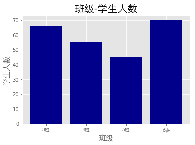
条形图
1
2
3
4
5
6
7
8
9
10
11
12
13
14
| 1import matplotlib.pyplot as plt
2from matplotlib.font_manager import FontProperties
3%matplotlib inline
4font = FontProperties(fname='/Library/Fonts/Heiti.ttc')
5
6# 修改背景为条纹
7plt.style.use('ggplot')
8
9classes = ['3班', '4班', '5班', '6班']
10
11classes_index = range(len(classes))
12print(list(classes_index))
13
14 |
1
2
3
4
5
6
7
8
9
10
11
12
13
14
15
16
17
18
19
20
| 1student_amounts = [66, 55, 45, 70]
2
3# 画布设置
4fig = plt.figure()
5# 1,1,1表示一张画布切割成1行1列共一张图的第1个;2,2,1表示一张画布切割成2行2列共4张图的第一个(左上角)
6ax1 = fig.add_subplot(1, 1, 1)
7ax1.bar(classes_index, student_amounts, align='center', color='darkblue')
8ax1.xaxis.set_ticks_position('bottom')
9ax1.yaxis.set_ticks_position('left')
10
11plt.xticks(classes_index, classes, rotation=0,
12 fontsize=13, fontproperties=font)
13plt.xlabel('班级', fontproperties=font, fontsize=15)
14plt.ylabel('学生人数', fontproperties=font, fontsize=15)
15plt.title('班级-学生人数', fontproperties=font, fontsize=20)
16# 保存图片,bbox_inches='tight'去掉图形四周的空白
17# plt.savefig('classes_students.png', dpi=400, bbox_inches='tight')
18plt.show()
19
20 |
直方图
1
2
3
4
5
6
7
8
9
10
11
12
13
14
15
| 1import numpy as np
2import matplotlib.pyplot as plt
3from matplotlib.font_manager import FontProperties
4%matplotlib inline
5font = FontProperties(fname='/Library/Fonts/Heiti.ttc')
6
7# 修改背景为条纹
8plt.style.use('ggplot')
9
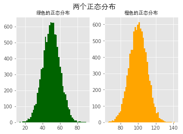
10mu1, mu2, sigma = 50, 100, 10
11# 构造均值为50的符合正态分布的数据
12x1 = mu1+sigma*np.random.randn(10000)
13print(x1)
14
15 |
1
2
3
4
| 1[59.00855949 43.16272141 48.77109774 ... 57.94645859 54.70312714
2 58.94125528]
3
4 |
1
2
3
4
5
| 1# 构造均值为100的符合正态分布的数据
2x2 = mu2+sigma*np.random.randn(10000)
3print(x2)
4
5 |
1
2
3
4
| 1[115.19915511 82.09208214 110.88092454 ... 95.0872103 104.21549068
2 133.36025251]
3
4 |
1
2
3
4
5
6
7
8
9
10
11
12
13
14
| 1fig = plt.figure()
2ax1 = fig.add_subplot(121)
3# bins=50表示每个变量的值分成50份,即会有50根柱子
4ax1.hist(x1, bins=50, color='darkgreen')
5
6ax2 = fig.add_subplot(122)
7ax2.hist(x2, bins=50, color='orange')
8
9fig.suptitle('两个正态分布', fontproperties=font, fontweight='bold', fontsize=15)
10ax1.set_title('绿色的正态分布', fontproperties=font)
11ax2.set_title('橙色的正态分布', fontproperties=font)
12plt.show()
13
14 |
折线图
1
2
3
4
5
6
7
8
9
10
11
12
13
14
15
16
17
| 1import numpy as np
2from numpy.random import randn
3import matplotlib.pyplot as plt
4from matplotlib.font_manager import FontProperties
5%matplotlib inline
6font = FontProperties(fname='/Library/Fonts/Heiti.ttc')
7
8# 修改背景为条纹
9plt.style.use('ggplot')
10
11np.random.seed(1)
12
13# 使用numpy的累加和,保证数据取值范围不会在(0,1)内波动
14plot_data1 = randn(40).cumsum()
15print(plot_data1)
16
17 |
1
2
3
4
5
6
7
8
9
| 1[ 1.62434536 1.01258895 0.4844172 -0.58855142 0.2768562 -2.02468249
2 -0.27987073 -1.04107763 -0.72203853 -0.97140891 0.49069903 -1.56944168
3 -1.89185888 -2.27591324 -1.1421438 -2.24203506 -2.41446327 -3.29232169
4 -3.25010794 -2.66729273 -3.76791191 -2.6231882 -1.72159748 -1.21910314
5 -0.31824719 -1.00197505 -1.12486527 -2.06063471 -2.32852279 -1.79816732
6 -2.48982807 -2.8865816 -3.5737543 -4.41895994 -5.09020607 -5.10287067
7 -6.22018102 -5.98576532 -4.32596314 -3.58391898]
8
9 |
1
2
3
4
5
6
7
8
9
10
11
12
13
14
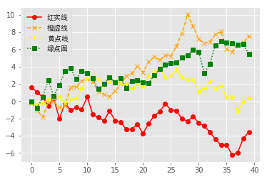
| 1plot_data2 = randn(40).cumsum()
2plot_data3 = randn(40).cumsum()
3plot_data4 = randn(40).cumsum()
4
5plt.plot(plot_data1, marker='o', color='red', linestyle='-', label='红实线')
6plt.plot(plot_data2, marker='x', color='orange', linestyle='--', label='橙虚线')
7plt.plot(plot_data3, marker='*', color='yellow', linestyle='-.', label='黄点线')
8plt.plot(plot_data4, marker='s', color='green', linestyle=':', label='绿点图')
9
10# loc='best'给label自动选择最好的位置
11plt.legend(loc='best', prop=font)
12plt.show()
13
14 |
散点图+直线图
1
2
3
4
5
6
7
8
9
10
11
12
13
14
15
| 1import numpy as np
2from numpy.random import randn
3import matplotlib.pyplot as plt
4from matplotlib.font_manager import FontProperties
5%matplotlib inline
6font = FontProperties(fname='/Library/Fonts/Heiti.ttc')
7
8# 修改背景为条纹
9plt.style.use('ggplot')
10
11
12x = np.arange(1, 20, 1)
13print(x)
14
15 |
1
2
3
| 1[ 1 2 3 4 5 6 7 8 9 10 11 12 13 14 15 16 17 18 19]
2
3 |
1
2
3
4
5
6
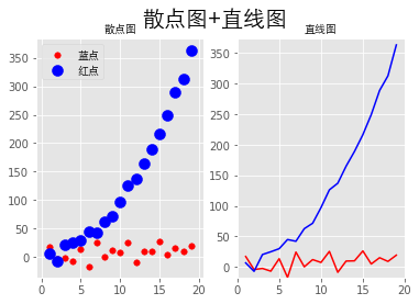
| 1# 拟合一条水平散点线
2np.random.seed(1)
3y_linear = x+10*np.random.randn(19)
4print(y_linear)
5
6 |
1
2
3
4
5
6
| 1[ 17.24345364 -4.11756414 -2.28171752 -6.72968622 13.65407629
2 -17.01538697 24.44811764 0.38793099 12.19039096 7.50629625
3 25.62107937 -8.60140709 9.77582796 10.15945645 26.33769442
4 5.00108733 15.27571792 9.22141582 19.42213747]
5
6 |
1
2
3
4
5
| 1# 拟合一条x²的散点线
2y_quad = x**2+10*np.random.randn(19)
3print(y_quad)
4
5 |
1
2
3
4
5
6
| 1[ 6.82815214 -7.00619177 20.4472371 25.01590721 30.02494339
2 45.00855949 42.16272141 62.77109774 71.64230566 97.3211192
3 126.30355467 137.08339248 165.03246473 189.128273 216.54794359
4 249.28753869 288.87335401 312.82689651 363.34415698]
5
6 |
1
2
3
4
5
6
7
8
9
10
11
12
13
14
15
16
17
18
19
20
| 1# s是散点大小
2fig = plt.figure()
3ax1 = fig.add_subplot(121)
4plt.scatter(x, y_linear, s=30, color='r', label='蓝点')
5plt.scatter(x, y_quad, s=100, color='b', label='红点')
6
7ax2 = fig.add_subplot(122)
8plt.plot(x, y_linear, color='r')
9plt.plot(x, y_quad, color='b')
10
11# 限制x轴和y轴的范围取值
12plt.xlim(min(x)-1, max(x)+1)
13plt.ylim(min(y_quad)-10, max(y_quad)+10)
14fig.suptitle('散点图+直线图', fontproperties=font, fontsize=20)
15ax1.set_title('散点图', fontproperties=font)
16ax1.legend(prop=font)
17ax2.set_title('直线图', fontproperties=font)
18plt.show()
19
20 |